Gaussian Elimination.

The Paragon message-passing library was instrumented to enable tracing and replaying all messages. The broadcasts were recorded as M_pivot and the the reads of the broadcasts were recorded as R_pivot. These events were then used as the basis for modeling the system's behavior. The communication behavior during elimination can then be modeled simply as:
ch pivot = M_pivot @ R_pivot;
This behavior is bound to the process set by the p-chain definition
set procset = { 0..8 };
pch iter = pivot onsome procset;
The first line defines procset to be the set of process ids (PIDs), in this case, the integers from 0 to 7. The second line defines a p-chain iter that binds the process behavior to a nonempty subset of processes as indicated by the keyword onsome.

The entire behavior of the program - a sequence of iterations - is defined by
set procset = { 0..8 };
ch pivot = M_pivot @ R_pivot;
pch iter = pivot onsome procset;
match gauss = < iter >;
where match here indicates that 7 instances of the p-chain iter are to be matched in the execution trace and assigned to the variable gauss; the angular brackets indicate the logical relation of precedes must hold between successive instances. Figure shows the result of the match.

Match trees are generally quite large; even in this simple example, the full tree has 81 nodes. As we mentioned earlier, Ave automatically compresses trees both horizontally (by eliding sibling nodes) and vertically (by pruning levels) for visualization. Suppressed sibling nodes are represented by a single node with button that can be used for scrolling through hidden constituents; an integer label gives the number of these constituents. Vertical compression is indicated by a summarizing box. Here, the tree is expanded only to the p-chain level as indicated by the boxes below each p-chain. Each box represents an entire subtree rooted at the p-chain node. It is labeled with an integer pair: the first component indicates the total number of behaviors (that is, the number of direct descendents of the p-chain node) and the second component indicates the number of different behaviors. In this case, one process participated in the first iteration and thus the number of behavior is inevitably one. The summarizing label was 1,1. Since in this case, only one process performed a broadcast in each iteration, the summarizing label is always 1,1. The user can get a description of the partitioning by clicking on the summarizing node as shown in Figure . Here the user clicked on the first summarizing node labeled 1,1 (as indicated by the black shading) to get the further information that it was process 0 who sent the broadcast as was expected.

The match tree in the figure shows an unsuccessful model match as indicated by the error message

Precedes failed between highlighted abstract events

This means that although the expected chains occurred in the execution history graph, the expected logical relations, in this case precedes, did not hold between them. The highlighting (in bold italics) on the first two instances of iter indicates the first place in which it failed to hold.

The event-based debugging points to a bug at a high level of abstraction, but does not tell us the actual location of the bug in the source code. This is to be expected, since the user forms a higher level mental picture of the behavior, where each abstract event may contain several lines of source code. In order to find out where the actual fault lies, the user should have the opportunity to set a global breakpoint at or before the occurence of the high level error. This can be done in Ave/Ariadne by selecting the first abstract event iter, and giving the command
break after select;
which asks the debugger to set the breakpoint after the first iter abstract event . select is a keyword which always point to the abstract event selected by the user with the mouse, break and after are also keywords that are self-explanatory.

The re-execution under replay provided the following source window output as shown in Figure , where source lines with processes waiting on them are highlighted. A separate output identifies the processes that are waiting on particular source lines as shown in Figure . Another window displays the messages that were most recently seen (in case of local breakpoints immediately after a message event) or that are about to be encountered (in case of local breakpoints immediately before a message event). The messages are reproduced below:

==1.5-=.9=

Process 0 stopped after sending multicast message.
Process 1,2,3,4 stopped after receiving message from process 0.
Process 5 stopped before receiving message from process 2.
Process 6 stopped before receiving message from process 3.
Process 7 stopped before receiving message from process 6.

The description W R says that the pattern has two events W and R, and they happen in the same process, and are thus connected by a program order happened before edge. Note without any other qualification, such program order edge is also immediate.

The description W @ R says that the pattern has two events W and R and they happen in different processes and are connected by a causal order happened before edge. Causal order edges are always immediate.

The description of such relationship between events is accomplished via the mechanism of chains. Formally, a chain is a tree that is to be matched against the execution history graph. Nodes in the tree can represent communication events: ReadEvents denoted by R, or WriteEvents, denoted by either W or M (depending on whether it is a single write or a multicast), Events can be suffixed with explicit tags such as W_pivot and R_elim.

The matching process for a chain always begins on a single process. It may stay entirely on that process, as in the above examples, or it may migrate to other processes by following a communication arc. An @ occurring between a WriteEvent and a ReadEvent event denotes a migration; matching is suspended on the writing process and initiated on the receiving process. Thus, c = W @ R defines a pattern in which the W is matched on the initiating process and the R is matched on the receiving process. Similarly,
W @ R W
describes a pattern in the first W is matched on the initiating process and the remaining R and W are matched on the receiving process. If a M precedes an @, matching is simultaneously initiated on all receiving processes.

Once matching has been completed on the receiving process(es), it may resume on the writing process where it had been suspended. If this is the case, it is indicated by ``marking'' the point of return before migration with the symbol <@. The symbol @> indicates that the matching should return to the most recent process on which it had been suspended, at the point of suspension. Thus B <@ R @> + B @ R models two consecutive multicasts on a single process; in the first case, the matching control returns to the initiating process, in the second it does not.

We can also define a tree structure at the chain level. Every time we encounter a @, we follow a graph edge to a different process, and start matching events in the receiving processes timeline. This kind of traversal of process timeline may happen multiple times depending on the pattern description. In case, the user wishes to return to a process timeline later, he/she needs to explicitly save the process information. At a later stage in the matching (in the regular expression) the user can then ask the saved information to be used to restore the matching context to the earlier process timeline. : saves the context of the process on a stack, and : asks the debugger to reset the matching context to the timeline of the process stored at the top of the stack.

With hierarchical behavioral description, behaviors can be partitioned across different hierarchical levels, all of which may or may not make sense to the user. So Ave only provides a default partitioning at the spatial domain (i.e., partition the processors that are involved in different behaviors at the p-chain level), which has already been described. The user retains the ability to partition behaviors across any level, with respect to the intrinsic (or derived) attributes of the abstract events of that level.

A new partition imposes an additional structure on the tree, which can be thought of as a structural transformation of the match tree. The user can investigate the behavior through this new structural transformation: A partition is thus equivalent to the imposition of multiple views on the program behavior []. We provide a uniform interface for such structural transformation. The following example outlines the structural transformation through incremental attribute computation and set partitioning.

Consider the scattering example once again. Suppose each processor always sends atleast 2 messages in each phase: atleast one message to an even-numbered processor, and atleast one to an odd-numbered processor. The user may be interested in looking into the messages sent to the odd-numbered processors only, and thus would like to partition the behavior along this attribute.

Figure already shows the attribute dest computed, in order to find out whether messages were truly scattered (sent to distinct processors). Now we can compute a new attribute that says whether the messages were sent to odd or even numbered processors. The command is as follows:
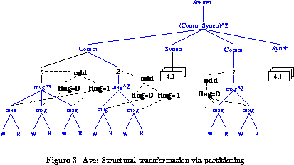
? with Scatter foreach msg compute flag = dest(msg) mod 2;
This adds a new attribute flag to each node named msg, which is set to 1 if the message was sent to a odd processor, or 0 if it was sent to an even processor. The user can then partition the behavior, to impose a structural transformation:
? with Scatter foreach proc create partition odd wrt flag;
This adds a new structure to the tree. The new nodes are shown in bold font, and the resulting additional tree structure is shown with dashed lines in Figure .

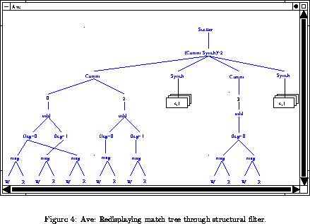
If the user chooses to display the tree through this new structural transformation, the tree in Figure will be displayed.

With hierarchical behavioral description, behaviors can be partitioned across different hierarchical levels, all of which may or may not make sense to the user. So Ave only provides a default partitioning at the spatial domain (i.e., partition the processors that are involved in different behaviors at the p-chain level), which has already been described. The user retains the ability to partition behaviors across any level, with respect to the intrinsic (or derived) attributes of the abstract events of that level.

A new partition imposes an additional structure on the tree, which can be thought of as a structural transformation of the match tree. The user can investigate the behavior through this new structural transformation: A partition is thus equivalent to the imposition of multiple views on the program behavior [].